Examples of use
Example 1: Spin half Larmor precession
Full code
# Define field for spin system
def get_field_larmor(time_sample, sweep_parameters, field_sample):
    field_sample[0] = 0              # Zero field in x direction
    field_sample[1] = 0              # Zero field in y direction
    field_sample[2] = math.tau*1000  # Split spin z eigenstates by 1kHz

# Initialise simulator instance
simulator_larmor = spinsim.Simulator(get_field_larmor, spinsim.SpinQuantumNumber.HALF)
# Evaluate a simulation
results_larmor = simulator_larmor.evaluate(0e-3, 100e-3, 100e-9, 500e-9, spinsim.SpinQuantumNumber.HALF.plus_x)

# Plot results
plt.figure()
plt.plot(results_larmor.time, results_larmor.spin)
plt.legend(["x", "y", "z"])
plt.xlim(0e-3, 2e-3)
plt.xlabel("time (s)")
plt.ylabel("spin expectation (hbar)")
plt.title("Spin projection for Larmor precession")
plt.show()
Explanation
The most basic system that spinsim can simulate is that of Larmor precession of a spin-half system.
Here, the two spin z projection eigenstates are split by a source potential \(\omega_L\), measured in rad/s.
Note
In spinsim, energies are written in dimensions of angular frequency, in units of rad/s, where the value used is the frequency equivalent to the energy given by the Plank-Einstein relation, \(\omega = \frac{E}{\hbar}\), with \(\hbar\) being (reduced) Plank’s constant.
When the system is initialised in a state of definite spin z projection, it gains a phase over time. However, if the system is started in a superposition of these states, the expected spin projection (Bloch) vector will precess around the \(z\) axis at a rate of \(\omega_L\).
The first thing we need to do is import the correct packages for the example.
As well as spinsim for simulations, we will use math to access math.tau (ie the constant \(2\pi\)), and matplotlib.pyplot to plot our results.
import spinsim
import matplotlib.pyplot as plt
import math
When set to spin-half mode, the spinsim package solves time dependent Schroedinger Equations of the form
where \(i^2 = -1\), \(\psi(t) \in \mathbb{C}^2\), and the spin-half spin projection operators are given by
The source of the system is the collection of energy functions \(\omega_x(t), \omega_y(t), \omega_z(t)\), with \(t\) in units of s and \(\omega\) in units of rad/s that control the dynamics of the system. The user must define a function that returns a sample of these source functions when a sampling time is input. In physical terms, these functions would represent the \(x,y,z\) components of a magnetic field applied to an atom being simulated, for example.
To continue with our example, the Larmor system follows a Schroedinger equation of
so
Let’s pick \(\omega_L = 2\pi\cdot1\,\mathrm{kHz}\). We can write this as a python function as follows:
# Define field for spin system
def get_field_larmor(time_sample, sweep_parameters, field_sample):
    field_sample[0] = 0              # Zero field in x direction
    field_sample[1] = 0              # Zero field in y direction
    field_sample[2] = math.tau*1000  # Split spin z eigenstates by 1kHz
This function has three inputs.
time_sample and field_sample are the equivalent of \(t\) and \((\omega_x, \omega_y, \omega_z)\) from before.
In particular, field_sample is a numpy array of doubles, with indices 0, 1, 2 representing for indices \(x, y, z\) respectively.
sweep_parameters is a user input to the function, which we will explore in the next example.
We can then construct an object of spinsim.Simulator to return an integrator with this specific function built in.
# Initialise simulator instance
simulator_larmor = spinsim.Simulator(get_field_larmor, spinsim.SpinQuantumNumber.HALF)
This integrator is compiled for specific devices determined by the key word argument device, with choices from the values of the enum.Enum, spinsim.Device.
For example, if the user wants to run simulations using a multicore CPU, they can instead write
# Initialise simulator instance
simulator_larmor = spinsim.Simulator(get_field_larmor, spinsim.SpinQuantumNumber.HALF, device.CPU)
By default, the spinsim.Simulator instance checks whether or not Cuda (Nvidia GPU) devices are available, and if one is, it compiles the simulation code for Cuda compatible Nvidia GPUs to run in massive parallel.
This is the fastest way to run spinsim.
Otherwise, it compiles the simulation code for CPU (parallelised).
The compilation is done by the numba package.
This means that the function get_field() supplied by the user must be compilable for the desired device using numba.
See the documentation for spinsim.Device for more information on the restrictions this results in.
The constructor of spinsim.Simulator contains many other options that can be used to customise which features are used by the integrator.
The next step is to define some simulation parameters, as well as the input and output.
Firstly, we must decide on some time steps that are to be used.
time_step_output defines the resolution of the output time series for the time evolution operator, state and spin.
time_step_integration determines the internal time step of the integrator.
Note that time_step_output must be an integer multiple of time_step_integration.
We also need to define the times when the experiment starts and ends.
Below we have chosen to have a time_step_integration of 10ns, a time_step_output of 100ns, a start time of 0ms, and an end time of 100ms.
We also need to define an initial state for the spin system.
The eigenstates of the spin operators are provided as attributes to the spinsim.SpinQuantumNumber enums.
Alternatively, one can use a numpy.ndarray to input an arbitrary initial state.
We choose an eigenstate of the \(J_x\) operator spinsim.SpinQuantumNumber.HALF.plus_x, as we expect that to precess as it evolves through time.
Now that everything is set up, the time evolution operator can be found between each sample using our object simulator_larmor.
We can now run the simulation.
# Evaluate a simulation
results_larmor = simulator_larmor.evaluate(0e-3, 100e-3, 100e-9, 500e-9, spinsim.SpinQuantumNumber.HALF.plus_x)
Has this worked? We can plot the results using matplotlib.pyplot (zoomed in to show details),
# Plot result
plt.figure()
plt.plot(results_larmor.time, results_larmor.spin)
plt.legend(["x", "y", "z"])
plt.xlim(0e-3, 2e-3)
plt.xlabel("time (s)")
plt.ylabel("spin expectation (hbar)")
plt.title("Spin projection for Larmor precession")
plt.show()
which results in
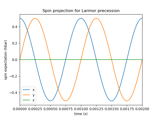
Here we see that indeed, the bloch vector is precessing anticlockwise at a frequency of 1kHz around the positive z axis.
Example 2: Time dependent field and sweeping parameters
Full code
import spinsim
import matplotlib.pyplot as plt
import math

# Define field for spin system
def get_field_rabi(time_sample, sweep_parameters, field_sample):
    # Dress atoms from the x direction, Rabi flopping at 1kHz
    field_sample[0] = 2*sweep_parameters[1]*math.cos(sweep_parameters[0]*time_sample)
    field_sample[1] = 0                    # Zero field in y direction
    field_sample[2] = sweep_parameters[0]  # Split spin z eigenstates by 700kHz
    field_sample[3] = 0                    # Zero quadratic shift, found in spin-one systems

# Initialise simulator instance
simulator_rabi = spinsim.Simulator(get_field_rabi, spinsim.SpinQuantumNumber.ONE)
# Evaluate a simulation
result0 = simulator_rabi.evaluate(0e-3, 100e-3, 100e-9, 500e-9, spinsim.SpinQuantumNumber.ONE.plus_z, [math.tau*20e3, math.tau*1e3])
# Evaluate another simulation
result1 = simulator_rabi.evaluate(0e-3, 100e-3, 100e-9, 500e-9, spinsim.SpinQuantumNumber.ONE.plus_z, [math.tau*40e3, math.tau*1e3])

# Plot results
plt.figure()
plt.plot(result0.time, result0.spin)
plt.legend(["x", "y", "z"])
plt.xlim(0e-3, 2e-3)
plt.xlabel("time (s)")
plt.ylabel("spin expectation (hbar)")
plt.title("Spin projection for Rabi flopping (20kHz bias)")
plt.draw()
plt.figure()
plt.plot(result1.time, result1.spin)
plt.legend(["x", "y", "z"])
plt.xlim(0e-3, 2e-3)
plt.xlabel("time (s)")
plt.ylabel("spin expectation (hbar)")
plt.title("Spin projection for Rabi flopping (40kHz bias)")
plt.draw()

plt.show()
Explanation
Now that we have confirmed that the most basic quantum system can be simulated using spinsim, we can explore a more complicated system with varying parameters.
Again, we import some packages,
import spinsim
import matplotlib.pyplot as plt
import math
Let’s first introduce the Rabi system. As before, we split the energy levels of the spin system (which is now three levels), with an energy difference \(\omega_L\) between each consecutive level. Again, if started in an eigenstate of \(J_x\), the expected spin will precess anticlockwise around the positive z axis. Radiation can be applied to the system to drive transitions between the spin states. For this to work, radiation must be resonant (or close to resonant) with the energy splitting (ie, its frequency of oscillation must be close to \(\omega_L\)). If the system starts with the expected spin pointing completely up, this radiation will drive the system to point completely down. It will then drive the system back up, and the cycle repeats. This happens at a rate of half of the amplitude of the radiation (assuming perfect resonance), which is called the Rabi frequency \(\Omega_R\), and the cycling is called Rabi flopping. The Schroedinger equation of the Rabi system is
In general, spinsim can solve Schroedinger equations of the form
where now \(\psi(t) \in \mathbb{C}^3\), and the spin-one operators are given by
\(J_x, J_y, J_z\) are regular spin operators, and \(Q\) is a quadratic operator, proportional to \(Q_{zz}\) as defined by [HGH+12], and \(Q_0\) as defined by [DWW10].
Just as before, we must define a source function, this time being time dependent.
# Define field for spin system
def get_field_rabi(time_sample, sweep_parameters, field_sample):
    # Dress atoms from the x direction, Rabi flopping at 1kHz
    field_sample[0] = math.tau*2000*math.cos(math.tau*20e3*time_sample)
    field_sample[1] = 0              # Zero field in y direction
    field_sample[2] = math.tau*20e3  # Split spin z eigenstates by 20kHz
    field_sample[3] = 0              # Zero quadratic shift, found in spin-one systems
This time there is a fourth entry in field_sample, which represents the quadratic shift \(\omega_q(t)\).
Here we have chosen a Larmor frequency \(\omega_L\) of \(2\pi\cdot20\,\mathrm{kHz}\), and a Rabi frequency \(\Omega_R\) of \(2\pi\cdot1\,\mathrm{kHz}\).
Warning
Remember, these functions must be numba.cuda.jit() compilable.
Before we move on, it is common that we might want to execute multiple similar simulations.
For example, we could run the current simulation, then one that is exactly the same, but with double the Larmor frequency \(\omega_L\).
One could do this by hard coding another source function with this change and then compiling another solver, but this takes time and is inefficient.
Instead, we can use the user input sweep_parameters.
Here we use sweep_parameters[0] in place of the previously hard coded value for the Larmor frequency, and sweep_parameters[1] in place of the previously hard coded value for the Rabi frequency.
# Define field for spin system
def get_field_rabi(time_sample, sweep_parameters, field_sample):
    # Dress atoms from the x direction, Rabi flopping
    field_sample[0] = 2*sweep_parameters[1]*math.cos(sweep_parameters[0]*time_sample)
    field_sample[1] = 0                          # Zero field in y direction
    field_sample[2] = sweep_parameters[0]  # Split spin z eigenstates
    field_sample[3] = 0                          # Zero quadratic shift, found in spin-one systems
sweep_parameters is input as a numpy.ndarray, meaning any number of parameters can be swept over using a single instance of spinsim.Simulator.
In general, this can be used to sweep through values for any number of simulations, meaning less time is wasted on compilation.
Let’s build our simulator object, now spin-one.
# Initialise simulator instance
simulator_rabi = spinsim.Simulator(get_field_rabi, spinsim.SpinQuantumNumber.ONE)
We decide on evaluation arguments as before, and we are now ready to execute.
sweep_parameters is the final argument to spinsim.Simulator.evaluate().
It is optional, so if it is unused in your get_field function it can be left out, as it was in the previous example.
Here it is set to [math.tau*20e3, math.tau*1e3], for a Larmor frequency \(\omega_L\) of \(2\pi\cdot20\,\mathrm{kHz}\) and a Rabi frequency \(\Omega_R\) of \(2\pi\cdot1\,\mathrm{kHz}\).
# Evaluate a simulation
result0 = simulator_rabi.evaluate(0e-3, 100e-3, 100e-9, 500e-9, spinsim.SpinQuantumNumber.ONE.plus_z, [math.tau*20e3, math.tau*1e3])
Finally we can plot our results.
# Plot results
plt.figure()
plt.plot(result0.time, result0.spin)
plt.legend(["x", "y", "z"])
plt.xlim(0e-3, 2e-3)
plt.ylim(-1, 1)
plt.xlabel("time (s)")
plt.ylabel("spin expectation (hbar)")
plt.title("Spin projection for Rabi flopping (20kHz bias)")
plt.draw()
which gives
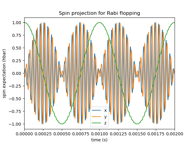
Notice the spin z projection cycling (Rabi flopping) at a rate of 1KHz, while the spin x and y projections are cycling between each other (Larmor precessing) at a rate of 20kHz. Using the rotating wave approximation, the spin z projection can be thought of as a sine wave. However, when these approximations are not used, one obtains these artifacts that we see on the spin z projection, known as beyond rotating wave effects.
Finally, let’s run another experiment using the same compiled function.
This will run faster than last time, as it does not need to be compiled a second time.
Here we set sweep_parameters to [math.tau*40e3, math.tau*1e3], for a Larmor frequency \(\omega_L\) of \(2\pi\cdot40\,\mathrm{kHz}\) and a Rabi frequency \(\Omega_R\) of \(2\pi\cdot1\,\mathrm{kHz}\).
This will double the Larmor frequency, and keep the Rabi frequency the same.
# Evaluate another simulation
result1 = simulator_rabi.evaluate(0e-3, 100e-3, 100e-9, 500e-9, spinsim.SpinQuantumNumber.ONE.plus_z, [math.tau*40e3])

# Plot result
plt.figure()
plt.plot(result1.time, result1.spin)
plt.legend(["x", "y", "z"])
plt.xlim(0e-3, 2e-3)
plt.xlabel("time (s)")
plt.ylabel("spin expectation (hbar)")
plt.title("Spin projection for Rabi flopping (40kHz bias)")
plt.draw()
which results in
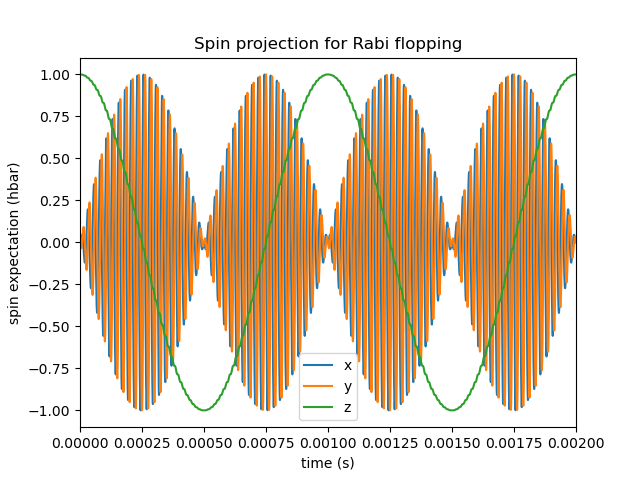
See that the spin projections are similar to last time, except that the Larmor precession is now at 40KHz.
Example 3: Gaussian Pi pulse and sampling
Full code
import spinsim
import math
import numpy as np
import matplotlib.pyplot as plt
import datetime as dtm

# Find the time
time_now_string = dtm.datetime.now().strftime("%Y%m%dT%H%M%S")

# Define the field function
def gaussian_pulse(time, sweep_parameters, pulse):
    pulse[0] = math.pi/math.sqrt(math.tau)*math.exp(-0.5*(time**2))
    pulse[1] = 0.0
    pulse[2] = 0.0

# Initialise plots
plt.figure()
legend = []
colours = ["r", "g", "b", "c", "m", "y"]

# Calculate the analytic solution
def cumulative_gaussian(t):
    return 0.5*(1 + math.erf(t/math.sqrt(2.0))) - 0.5*(1 + math.erf(-5.0/math.sqrt(2.0)))

time = np.arange(-5.0, 5.1, 2.0)
state_analytic = np.asarray([[math.cos(0.5*math.pi*cumulative_gaussian(t)), -1j*math.sin(0.5*math.pi*cumulative_gaussian(t))] for t in time], dtype = np.complex128)

# Initialise simulations
simulator = spinsim.Simulator(gaussian_pulse, spinsim.SpinQuantumNumber.HALF)
error = []
time_steps = np.asarray([0.001, 0.005, 0.01, 0.05, 0.1, 0.25, 0.5, 1.0, 2.0])
number_of_steps = 10 / time_steps
plot_start_index = 4

# Loop through simulations at different time steps
for simulation_index, time_step in enumerate(time_steps):
    # Simulate at a particular time step
    result_simulated = simulator.evaluate(-5.0, 7.0, time_step, 2.0, np.asarray([1, 0], np.complex128))

    # Calculate error
    error += [np.sqrt(np.sum(np.abs(result_simulated.state - state_analytic)**2))/5]

    # Plot spins
    if simulation_index >= plot_start_index:
        plt.plot(time, result_simulated.spin[:, 0], colours[simulation_index - plot_start_index] + "--o")
        plt.plot(time, result_simulated.spin[:, 1], colours[simulation_index - plot_start_index] + "--x")
        plt.plot(time, result_simulated.spin[:, 2], colours[simulation_index - plot_start_index] + "--+")

        legend += [
            "{:d} x".format(int(number_of_steps[simulation_index])),
            "{:d} y".format(int(number_of_steps[simulation_index])),
            "{:d} z".format(int(number_of_steps[simulation_index]))
        ]

# Calculate and plot analytic spins
time_smooth = np.arange(-5.0, 5.1, 0.02)
state_smooth = np.asarray([[math.cos(0.5*math.pi*cumulative_gaussian(t)), -1j*math.sin(0.5*math.pi*cumulative_gaussian(t))] for t in time_smooth], dtype = np.complex128)
spin_smooth = np.asarray([
    [
        (state_smooth[time_index, 0]*np.conj(state_smooth[time_index, 1])).real,
        (1j*state_smooth[time_index, 0]*np.conj(state_smooth[time_index, 1])).real,
        0.5*(state_smooth[time_index, 0].real**2 + state_smooth[time_index, 0].imag**2 - state_smooth[time_index, 1].real**2 - state_smooth[time_index, 1].imag**2)
    ] for time_index in range(time_smooth.size)
])

plt.plot(time_smooth, spin_smooth[:, 0], "k-")
plt.plot(time_smooth, spin_smooth[:, 1], "k-")
plt.plot(time_smooth, spin_smooth[:, 2], "k-")
legend += ["Analytic"]

plt.legend(legend, loc = "lower left")
plt.xlabel("Time (standard deviations)")
plt.ylabel("Spin")
plt.title("{}\nGaussian pulse at various numbers of steps".format(time_now_string))
plt.savefig("gaussian_pulse.png")
plt.savefig("gaussian_pulse.pdf")
plt.show()

# Plot errors for each time step
plt.figure()
plt.loglog(number_of_steps, error, "-rx")
plt.xlabel("Number of steps")
plt.ylabel("Error")
plt.title("{}\nError in integrating Gaussian pulse".format(time_now_string))
plt.savefig("gaussian_pulse_error.png")
plt.savefig("gaussian_pulse_error.pdf")
plt.show()

# Plot the sample locations used by the CF4 integrator at a resolution of 40 steps
plt.figure()
pulse_sample = np.empty(3, np.float64)

time_continuous = np.arange(-5.0, 5.0005, 1e-3)
pulse_continuous = []
for time_sample in time_continuous:
    gaussian_pulse(time_sample, 0, pulse_sample)
    pulse_continuous += [pulse_sample[0]]
pulse_continuous = np.asarray(pulse_continuous)
plt.plot(time_continuous, pulse_continuous, "k-")

time_step = 0.25
time_midpoint = 0.5*time_step + np.arange(-5.0, 5.0, time_step)
pulse_midpoint = []
for time_sample in time_midpoint:
    gaussian_pulse(time_sample, 0, pulse_sample)
    pulse_midpoint += [pulse_sample[0]]
pulse_midpoint = np.asarray(pulse_midpoint)
plt.plot(time_midpoint, pulse_midpoint, "bo")

time_quadrature = []
pulse_quadrature = []
for time_sample in time_midpoint:
    gaussian_pulse(time_sample - 0.5*time_step/math.sqrt(3), 0, pulse_sample)
    time_quadrature += [time_sample - 0.5*time_step/math.sqrt(3)]
    pulse_quadrature += [pulse_sample[0]]

    gaussian_pulse(time_sample + 0.5*time_step/math.sqrt(3), 0, pulse_sample)
    time_quadrature += [time_sample + 0.5*time_step/math.sqrt(3)]
    pulse_quadrature += [pulse_sample[0]]
time_quadrature = np.asarray(time_quadrature)
pulse_quadrature = np.asarray(pulse_quadrature)
plt.plot(time_quadrature, pulse_quadrature, "m.")

plt.xlabel("Time (standard deviations)")
plt.ylabel("Pulse strength (Hz)")
plt.legend(
    [
        "Pulse shape",
        "Integration steps",
        "Pulse sample points"
    ]
)
plt.title("{}\nSample points for integrating Gaussian pulse".format(time_now_string))
plt.savefig("gaussian_pulse_sample.png")
plt.savefig("gaussian_pulse_sample.pdf")
plt.show()
Explanation
This is a longer example, and benchmark, to show how spinsim can be used to accurately integrate pulses.
Here the spin system is acted on by a Gaussian pi pulse, which is a pulse in the shape of a Gaussian that rotates the Bloch vector (spin projection expectation) by 180 degrees.
In this case, this is modelled in the rotating frame, using the rotating wave approximation, as
Note that here we are only interested in the dynamics of the system in the rotating frame itself. One can simulate this system using spinsim with this python function
def gaussian_pulse(time, modifier, pulse):
    pulse[0] = (math.pi/math.sqrt(math.tau))*math.exp(-0.5*(time**2))
    pulse[1] = 0.0
    pulse[2] = 0.0
where the equation could be simplified if not for readability (the first pi is the rotation the Bloch vector is to make in radians, and the second is to normalise the Gaussian).
The code simulates the dynamics of this system at various time steps. The following shows the coarsely sampled spin projections for these differing accuracies,
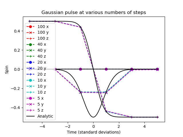
Notice how the Bloch vector rotates from pointing in the z direction, to pointing in the -y direction, and finally pointing in the -z direction after the pulse has completed. A 180 degree rotation has indeed been made.
The following shows how the accuracy of the evaluated state obtained relates to the integration step size used,
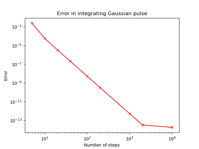
The flatline at \(10^{-14}\) is expected for any algorithm using the double-precision floating point data type, as that is where it reaches the limits of its precision. We find that using 40 steps across the whole -5 to +5 standard deviations of the Gaussian pulse results in an error in the state of less than \(10^{-6}\). The integration and time resolution can be seen in the following,
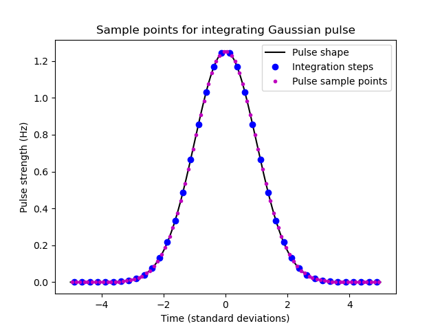
Time steps this coarse are able to be used because of the commutator free Magnus based integrator being used. Each step (in blue) uses two samples (in magenta) to sample the pulse shape (in black).
Example 4: Using the interpolator
This example introduces the interpolator generator that can be used to define the field function in terms of a sampled time series rather than mathematical functions. Some examples of the wide variety of tasks that can be done with this are:
Run simulations based off of magnetic field values already measured in your lab
Define smooth functions more complicated than those allowed with
numpyandmath…… including adding simulated noise to the system
Easily define a set of hard pulses in the rotating frame that turn on and off at arbitrary points in time…
… or use the output to modulate sinusoids and just run the hard pulse simulation in the lab frame instead
Similarly, easily define linear ramped pulses in the rotating and lab frames
In this example we focus on adding noise to the system. The process here is essentially the same as that for reading in recorded field amplitudes.
Full code
import spinsim
import matplotlib.pyplot as plt
import math
import numpy as np
# Generate noise
time_sampled = np.arange(0, 100e-3, 1e-3)
larmor_sampled = np.random.randn(time_sampled.size)
# Generate the interpolator
larmor_interpolator = spinsim.generate_interpolation_sampler(time_sampled, larmor_sampled)
def get_field_larmor_interpolator(time_sample, user_parameters, field_sample):
# We can vary the noise amplitude per simulation using user_parameters
noise_amplitude = user_parameters[0]
field_sample[2] = math.tau*(200 + noise_amplitude*larmor_interpolator(time_sample))
field_sample[0] = 0
field_sample[1] = 0
field_sample[3] = 0
# Simulate the system with first without noise, then with noise
simulator_larmor_interpolator = spinsim.Simulator(get_field_larmor_interpolator, spinsim.SpinQuantumNumber.ONE)
results_larmor = simulator_larmor_interpolator.evaluate(0, 100e-3, 1e-6, 10e-6, spinsim.SpinQuantumNumber.ONE.plus_x, [0])
results_larmor_interpolator = simulator_larmor_interpolator.evaluate(0, 100e-3, 1e-6, 10e-6, spinsim.SpinQuantumNumber.ONE.plus_x, [50])
# Visualise the interpolation
larmor_interpolator_plot = spinsim.generate_interpolation_sampler(time_sampled, larmor_sampled, device = spinsim.Device.CPU)
time_plot = np.arange(0, 100e-3, 100e-6)
larmor_plot = np.zeros(time_plot.size)
for time_index in range(time_plot.size):
larmor_plot[time_index] = 200 + 50*larmor_interpolator_plot(time_plot[time_index])
# Plot
plt.figure()
plt.plot(time_sampled, 200 + 50*larmor_sampled, "r.", label = "\"Recorded\" amplitudes")
plt.plot(time_plot, larmor_plot, "b-", label = "Interpolated amplitudes")
plt.xlabel("Time (s)")
plt.ylabel("Z field amplitude (Hz)")
plt.legend()
plt.ylim(0, 400)
plt.title("Noisy Larmor interpolation\nField timeseries")
plt.savefig("interpolation_example_1_timeseries.png")
plt.savefig("interpolation_example_1_timeseries.pdf")
plt.draw()
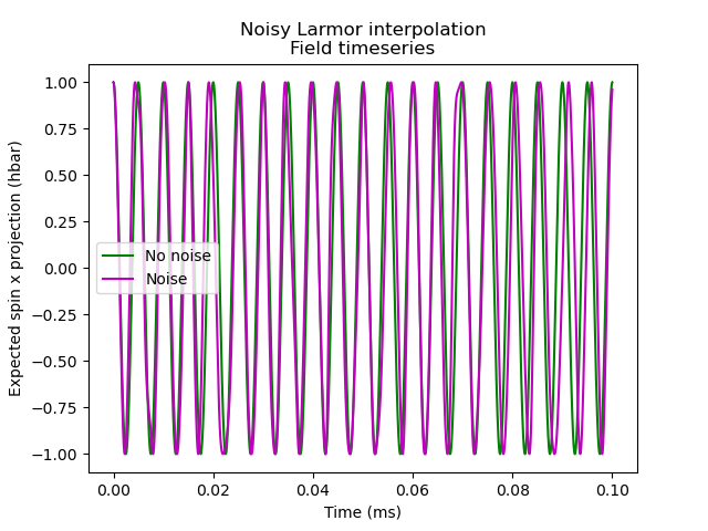
plt.figure()
plt.plot(results_larmor_interpolator.time, results_larmor.spin[:, 0], "g-", label = "No noise")
plt.plot(results_larmor_interpolator.time, results_larmor_interpolator.spin[:, 0], "m-", label = "Noise")
plt.xlabel("Time (ms)")
plt.ylabel("Expected spin x projection (hbar)")
plt.legend()
plt.title("Noisy Larmor interpolation\nField timeseries")
plt.savefig("interpolation_example_1_results.png")
plt.savefig("interpolation_example_1_results.pdf")
plt.draw()
plt.show()
Explanation
After importing some standard libraries, we generate some white (up to the sampling frequency) using numpy.random.randn.
In this way we generate an array amplitude_sampled that is IID and follows \(N(0, 1)\).
Because the interpolator works with a non-uniform sampling rate, we also need to define an array of sampling times time_sampled.
time_sampled = np.arange(0, 100e-3, 1e-3)
larmor_sampled = np.random.randn(time_sampled.size)
Next, we simply enter this time and amplitude data into spinsim.generate_interpolation_sampler, which returns a callable that can be used within a get_field function.
larmor_interpolator = spinsim.generate_interpolation_sampler(time_sampled, larmor_sampled)
Now we can define such a function.
Here we are simulating basic Larmor precession again, but with our simulated noise on top of the bias value.
Since the generated noise is mean zero and standard deviation one, we use user_parameters[0] to scale it and define the noise amplitude (or just turn it off).
def get_field_larmor_interpolator(time_sample, user_parameters, field_sample):
    # We can vary the noise amplitude per simulation using user_parameters
    noise_amplitude = user_parameters[0]
    field_sample[2] = math.tau*(200 + noise_amplitude*larmor_interpolator(time_sample))

    field_sample[0] = 0
    field_sample[1] = 0
    field_sample[3] = 0
Next, we define our spinsim.Simulator object and evaluate.
We simulate once with no noise (user_parameters = [0]) and once with a noise amplitude of 50 Hz for comparison (user_parameters = [50]).
simulator_larmor_interpolator = spinsim.Simulator(get_field_larmor_interpolator, spinsim.SpinQuantumNumber.ONE)
results_larmor = simulator_larmor_interpolator.evaluate(0, 100e-3, 1e-6, 10e-6, spinsim.SpinQuantumNumber.ONE.plus_x, [0])
results_larmor_interpolator = simulator_larmor_interpolator.evaluate(0, 100e-3, 1e-6, 10e-6, spinsim.SpinQuantumNumber.ONE.plus_x, [50])
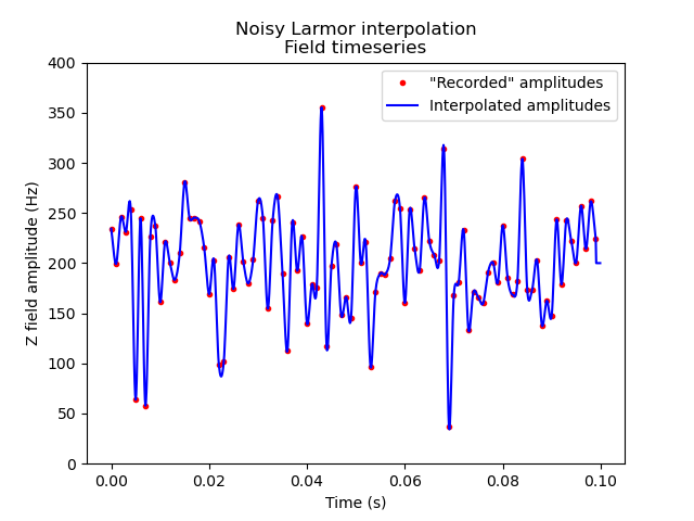
We are just about ready to plot our results, but before we do so, we may well like to plot what the interpolator is doing as well.
If we are using spinsim.Device.CUDA as the device for the interpolator to compile to (the default if a cuda compatible GPU is found on the system), then this cannot be done directly in python with the interpolator we defined before (unless you want to write a GPU kernel in numba.cuda to do so).
This is because the interpolator will only work on GPU.
Luckily, we can still see what the interpolator is doing by compiling it for CPU instead by setting the optional device argument to spinsim.Device.CPU.
larmor_interpolator_plot = spinsim.generate_interpolation_sampler(time_sampled, larmor_sampled, device = spinsim.Device.CPU)
time_plot = np.arange(0, 100e-3, 100e-6)
larmor_plot = np.zeros(time_plot.size)
for time_index in range(time_plot.size):
    larmor_plot[time_index] = 200 + 50*larmor_interpolator_plot(time_plot[time_index])
Finally we can plot the interpolator visualisation, as well as out simulation results.
plt.figure()
plt.plot(time_sampled, 200 + 50*larmor_sampled, "r.", label = "\"Recorded\" amplitudes")
plt.plot(time_plot, larmor_plot, "b-", label = "Interpolated amplitudes")
plt.xlabel("Time (s)")
plt.ylabel("Z field amplitude (Hz)")
plt.legend()
plt.ylim(0, 400)
plt.title("Noisy Larmor interpolation\nField timeseries")
plt.savefig("interpolation_example_1_timeseries.png")
plt.savefig("interpolation_example_1_timeseries.pdf")
plt.draw()

plt.figure()
plt.plot(results_larmor_interpolator.time, results_larmor.spin[:, 0], "g-", label = "No noise")
plt.plot(results_larmor_interpolator.time, results_larmor_interpolator.spin[:, 0], "m-", label = "Noise")
plt.xlabel("Time (ms)")
plt.ylabel("Expected spin x projection (hbar)")
plt.legend()
plt.title("Noisy Larmor interpolation\nField timeseries")
plt.savefig("interpolation_example_1_results.png")
plt.savefig("interpolation_example_1_results.pdf")
plt.draw()

plt.show()
We can see that the interpolator is using cubic interpolation (the default) to smoothly move between sampled values.
When noise is added to the simulation, the output begins to differ from what we expect.